How To Use Cell Values For Excel Chart Labels
 Image Credits: Howtogeek
You can turn your chart into labels in Microsoft Excel dynamic by linking them to individual cell values. When the data in the cell changes, the chart labels would automatically update itself. In this article, we would show you how to make both your chart title and the chart data labels to become dynamic.
We have the sample data below with the product their sales entries and the difference in the past month’s sales.
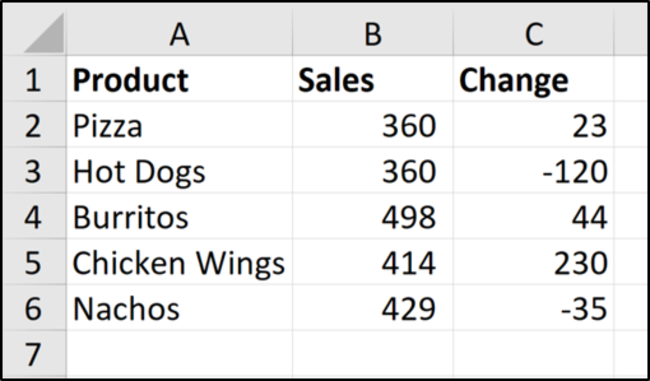 Image Credits: Howtogeek
Now, we want to create a chart of the sales values and use the changed values for data labels.
Use Cell Values for Chart Data Labels
Select a range A1:B6 and click on Insert > Insert Column or Bar Chart > Clustered Column.
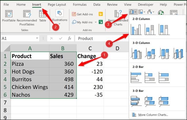 Image Credits: Howtogeek
The column chart will come up immediately after. Now, we would want to add data labels to show the change in value for each product compared to last month's data.
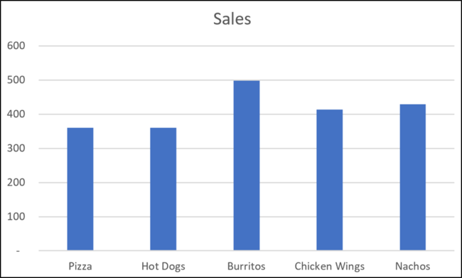 Image Credits: Howtogeek
Choose the chart, select the “Chart Elements” option, then click on the “Data Labels” arrow, and then “More Options.”
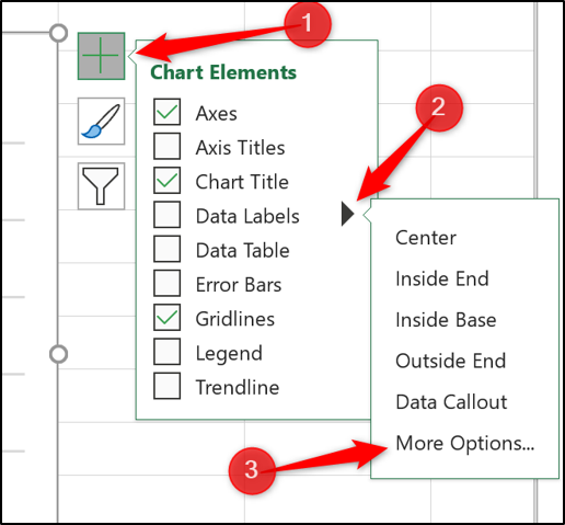 Image Credits: Howtogeek
Uncheck the “Value” box that follows and check the box that represents “Value From Cells.”
 Image Credits: Howtogeek
Select the cells C2:C6 to be used for the data label range and then click on the “OK” button.
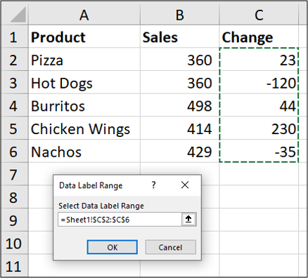 Image Credits: Howtogeek
The values from these cells would now be used for the chart data labels. If the values that are contained in these cells changes, then the chart labels will be automatically updated.
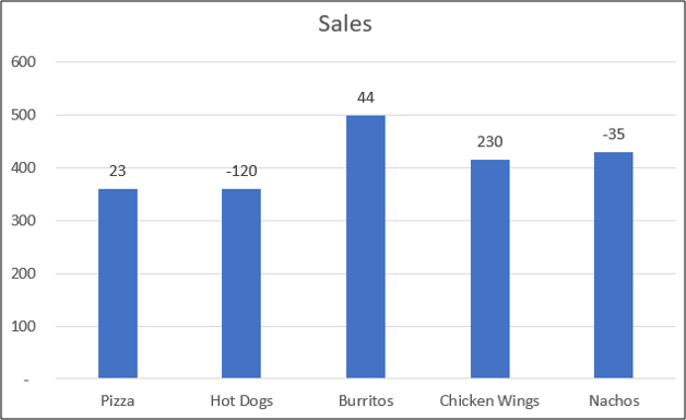 Image Credits: Howtogeek
Link a Chart Title to a Cell Value
In addition to the data labels, we would also want to link the chart title as well to a cell value to get something that is more dynamic and creative. We will start this tutorial by developing a useful chart title in a cell. We would then want to show the total sales in the chart title.
In cell E2, enter the below formula:
="Monthly Sales Total - "&TEXT(SUM(B2:B6),"0,###")
This formula would create a useful title that joins together the text “Monthly Sales Total – ” to the sum of values in B2: B6.
The TEXT in Excel function is used to format the number with a thousands separator.
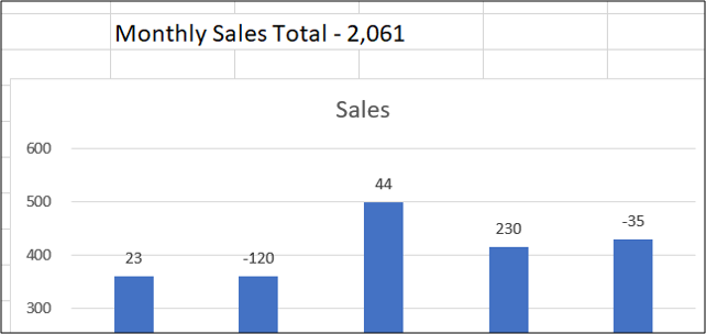 Image Credits: Howtogeek
We now need to link the chart title to the cell E2 to be able to use the text that we have created.
Click the chart title, then enter = into the Formula Bar, and then click on the cell E2. From there, press the Enter key.
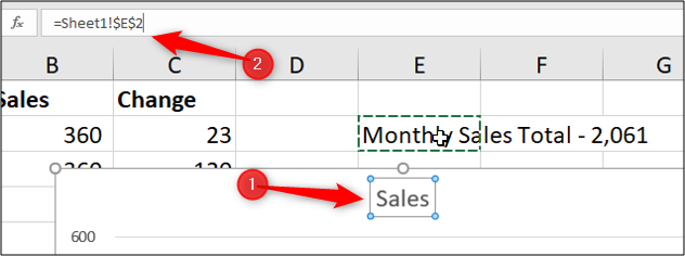 Image Credits: Howtogeek
After that, you would notice that the value from cell E2 would then be used for the chart title.
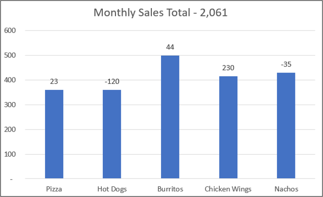 Image Credits: Howtogeek
If the values that are stored in the data range were to change, you would see that our data labels and our chart title would be also updated to reflect the new values on the chart.
By using both dynamic and creative labels for your charts, by basing them on cell values, you would take your charts beyond the standard charts that others create in Microsoft Excel.