How To Use VLOOKUP In Excel
What is VLOOKUP in Excel?
In Excel, the VLOOKUP function is used to locate a specific piece of information within a table or data set and extract the corresponding data/information. In simple terms, the VLOOKUP function instructs Excel to "look for this piece of information (for example, bananas) in this data set (a table) and return some corresponding information about it (for example, the banana price").
VLOOKUP Formula
=VLOOKUP(lookup_value, table_array, col_index_num, [range_lookup])
To put it simply, the formula is saying, "Look for this piece of information in the following area and provide me with the corresponding data from another column."
The following arguments are passed to the VLOOKUP function:
1. Lookup_value (required argument) – Lookup value specifies the value in the first column of a table that we want to look up.
2. Table_array (required argument) – The table array contains the data to be searched. The VLOOKUP function performs a search in the array's left-most column.
3. Col_index_num (required argument) – This is an integer indicating the column number of the supplied table array from which you wish to retrieve a value.
4. Range_lookup (optional argument) – This parameter specifies what this function should return if it cannot find an exact match for the lookup value. The argument may be set to TRUE or FALSE, indicating the following:
TRUE – Approximate match; if no exact match is found, the closest match below the lookup value is used.
FALSE – Exact match; if an exact match is not found, an error is returned.
How to use VLOOKUP in Excel
The first step is to organize the data
To use the VLOOKUP function effectively, the first step is to ensure that your data is well organized and suitable for the function.
Because VLOOKUP operates in a left-to-right direction, you must ensure that the information you wish to look up is to the left of the data you wish to extract.
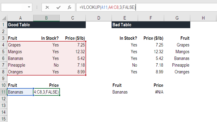
For instance:

As demonstrated in the preceding VLOOKUP example, the "good table" can easily execute the function to look up "Bananas" and return their price, as Bananas are located in the leftmost column. As you can see in the "bad table" example, there is an error message because the columns are not in the correct order.
This is a significant disadvantage of VLOOKUP, and it is strongly recommended that you use INDEX MATCH instead.
Second step is to instruct the function to perform a lookup
This step instructs Excel on what to look for. We begin by typing the formula "=VLOOKUP(" and then selecting the cell containing the data to be looked up. In this case, it is the cell containing the word "Bananas."
Third step is to instruct the function to look in the specified location
In this step, we select the table containing the data and instruct Excel to search for the information we selected in the previous step in the leftmost column.
For instance, we highlight the entire table from column A to column C in this case. Excel will look up the data we specified in column A.
Next step is to instruct Excel to output data from the specified column
This step instructs Excel on which column contains the data we want to output from the VLOOKUP. Excel requires a number that corresponds to the column number in the table to accomplish this.
Because the output data is in the third column of the table in our example, we enter the number "3" in the formula.
Lastly, instruct Excel to look for accurate or imprecise match
By specifying "True" or "False" in the formula, you can inform Excel whether you're looking for an exact or approximate match.
We want an exact match ("Bananas") in our VLOOKUP example, so we type "FALSE" in the formula. If we instead used the parameter "TRUE," we would get a close match.
An approximate match is useful when looking up an exact figure that is not included in the table, such as 2.9585. In this case, Excel will search for the closest value to 2.9585, even if that value is not present in the dataset. This will assist in preventing VLOOKUP formula errors.

