How To Filter Charts In Excel

You may wish to disable specific sections of your chart from view in order to concentrate on specific data at various points. This is made possible through the application of filters.

How to Sort and Filter a Chart

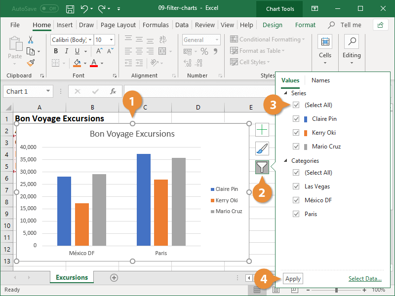
1. Begin by selecting the chart you wish to filter from the dropdown menu.

2. From the drop-down menu, select the Chart Filters option.

3. Select the item(s) that you want to show or hide.

4. Press the Apply button to save your changes.

The worksheet retains all of the information, but only the values that were selected appear in the chart.

Remove a Filter 

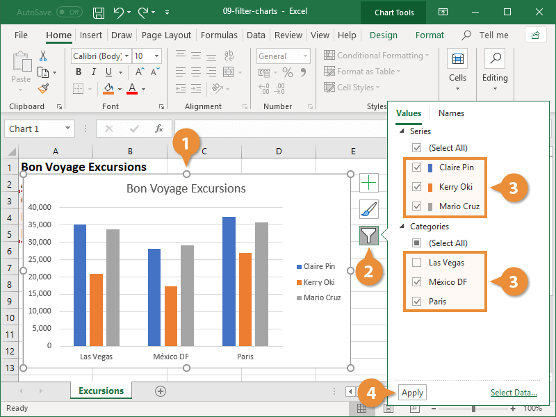
When you need access to all of your data again, simply remove the filter.

1. Find the chart that contains the filter that you want to remove and click on it.

2. From the drop-down menu, select the Chart Filters option.

3. To see the data that has been filtered, double-click the Select All check box.

4. Press the Apply button to save your changes.