How To Identify And Remove Duplicates From An Excel Spreadsheet (3 Easy Ways)

How to Identify and Remove Duplicates from an Excel Spreadsheet (3 Easy Ways)

For the purpose of this article, we'll examine three straightforward methods for removing or deleting duplicates in Excel:

1. Using the Remove Duplicates command located on the Data tab of the Ribbon.

2. Table Design or Table Tools Design tabs of the Ribbon contain a command called Remove Duplicates.

3. If the data contains extra spaces, a formula should be created to eliminate duplicates.

Identification of duplicate rows and subsequent deletion of those rows is the procedure.

The following items should be included in the list or data set for each of the techniques described further below:

• Header row headers that are distinct from one another
• There are no blank rows in this table.
• There are no blank columns in this table.
• There are no cells that have been merged.

In the event that you used the Subtotal feature to create subtotals, you should remove them. The use of spaces in the field names of Excel tables is discouraged if you intend to use structured reference formulas in your spreadsheets.

Note: Although the screenshots in this article were taken from Excel 365, they are comparable to those taken from previous versions of Excel.

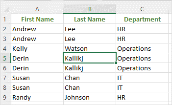
A sample data set is provided below, which contains unique headers as well as duplicate records; however, there are no blank rows or columns:

Preferably, you should save a copy of the worksheet or workbook before deleting any duplicates in order to ensure that all of the original data is retained.

 

1. Using Remove Duplicates on the Data tab of the Ribbon to remove duplicates from the database

To remove or delete duplicates from a data set using the Remove Duplicates command on the Ribbon, perform the following steps:

1. Select a cell in the data set or list that contains the duplicates you wish to remove from the data set or list. If the data set contains blank rows or columns, you must first select the data from the data set and then run the query (click in the first cell and Shift-click in the last cell).

2. Select the Data tab from the Ribbon navigation bar.

3. Select Remove Duplicates from the Data Tools drop-down menu. A dialog box appears on the screen.

4. When your data set or list contains headers, select the checkbox labeled My data contains headers from the drop-down menu.

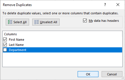
5. In the columns area, select or check the field(s) containing the duplicates you wish to remove. A single field (column) or all of the fields can be selected (columns). It appears that a dialog box has been opened that informs you of the number of records that will be deleted.

6. Press the OK button to confirm your action.

In this case, Excel will eliminate duplicate records while keeping the first row of each duplicate record and providing a summary of the rows that were removed.

Using a keyboard shortcut, you can quickly access the Remove Duplicates command on the Data tab of the Ribbon by pressing Alt > A > M. (Press Alt, then A, then M to get started.)

Remove Duplicates is a tool that can be found in the Data Tools group on the Data tab of the Ribbon:

In the Remove Duplicates dialog box, three fields from the data set are displayed. These are as follows:

 

2. Removing duplicates from an Excel spreadsheet

The Table Design and Table Tools Design tabs on the Ribbon can be used to eliminate duplicates if your data has been formatted as an Excel table (which is typically accomplished by pressing Ctrl + T).

The following steps should be followed in order to eliminate duplicates from an Excel table:

1. Select the table that contains the duplicates you wish to remove from the system.

2. To begin, select the Table Design or Table Tools Design tab from the Ribbon menu.

3. Select Remove Duplicates from the Tools drop-down menu. A dialog box appears on the screen.

4. If your table contains headers, select the checkbox labeled My data contains headers from the drop-down menu.

5. In the columns area, select or check the field(s) containing the duplicates you wish to remove. A single field (column) or all of the fields can be selected (columns). It appears that a dialog box has been opened that informs you of the number of records that will be deleted.

6. Press the OK button to confirm your action.

Excel will remove any duplicate rows and provide a summary of the total number of rows that have been removed from the worksheet.

Remove Duplicates is a tool that can be found in the Tools group on the Table Design or Table Tools Design tab of the Ribbon:

Also available on the Data tab is the Remove Duplicates command, which allows you to eliminate duplicates from a database.

 

3. Using a formula to remove duplicates 

In order to assist you in identifying duplicates that may contain additional spaces and thus are not recognized as such, you can enter a formula into the field.

The strategy that will be implemented is as follows:

• The TRIM function, which eliminates blank spaces between words as well as leading and trailing spaces.
• It is possible to join cells together by using the CONCATENATE operator (&). (although you can use the CONCATENATE or CONCAT functions as well)

For the Remove Duplicates command to work, you must first create a new calculated column (also known as a helper column) in your data.

To combine the information in cells A2 and B2 while eliminating any extra spaces in a cell (such as C2), you could use the following formula:

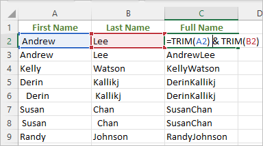
= TRIM(A2) & TRIM (B2)

If we look at the following example (which contains both first and last names), we can see that we entered the formula =TRIM(A2) & TRIM(B2) in cell C2 and then copied it down to the cells below by dragging the Fill handle located in the lower right corner of the cell:

Using the following formula in the first data cell of a new calculated column as a structured reference formula that refers to field names will allow you to combine cells from columns in a table (which includes columns for first and last names) and eliminate unnecessary spaces: If you want to combine cells from columns in a table (which includes columns for first and last names and columns for other information), you can use the following formula as a structured reference formula that refers to field names:

=TRIM([@[First Name]]) & TRIM([@[Last Name]]) 

As soon as you press the Enter key, Excel will populate the entire column with the formula you entered.

The structured reference formula is entered in C2 using the TRIM and CONCATENATE operators, and the references are color coded in Excel using the following formula:

As long as the field names do not contain any spaces, you can enter the following equation in cell C2 of the table:

=TRIM([@FirstName]) and TRIM([@LastName])

In order to remove duplicates after creating a helper or calculated column, first click in the data set or table, and then select only the calculated column in the Remove Duplicates dialog box (as described above).